Sometimes you hear that a buy-and-hold investment strategy is superior to market timing.
I want to test this hypothesis. Let us consider the following simplified situation where we can invest in either the S&P500 or in a money market account with a fixed yearly return of 3%. The goal is to find a market timing strategy that would yield a higher return than a buy-and-hold of the S&P500. Moreover, I assumed that the market timing decision can only be based on the evolution of the S&P500 up to that point in time. I am thus not using other data besides the S&P500 to time the market.
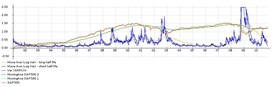
In the graph below you see the input data in red (historic S&P500 data over 20y). Derived from this data, in green are two moving averages averages. In blue is the S&P500 volatility, with in black and and yellow moving averages on the volatility.
Some market timing strategies based on this data come to mind:
Moving average crossovers consider two moving averages with different periods. The moving average with the shorter period will follow the data more closely, and will also be less smooth. If the S&P500 is on a mostly upward trajectory the moving average with the shorter period will be higher in value than the other moving average. However, if there are some declines of the market, the shorter moving average will follow this decline more closely. As such it will drop below the moving average with the longer period. This crossover of moving averages is sometimes used as an indicator to sell. The other type of crossover where they cross the other way signals a buying opportunity.
The strategy that I will consider further in this post, is another type of strategy based on the volatility. During periods of market stress the volatility shoots up. To determine whether the volatility is low or high, we compare it to a moving average of the volatility. Thus, on the above graph we consider the blue and black lines. If the blue line is above the trailing black then we consider it to be a period of market stress and move our investments to the safer money market account.
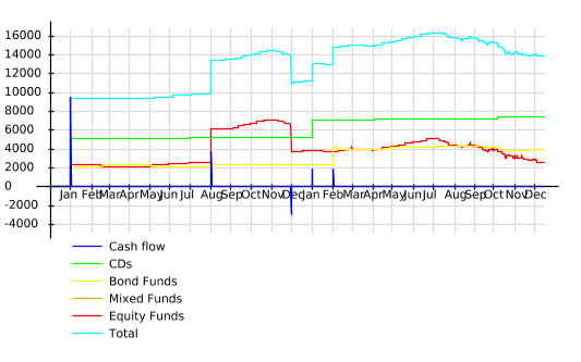
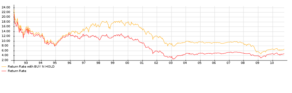
This strategy is represented in the chart below. The red indicates the amount held in the market, while the black line is the money held in the money market account. The total return is given in light blue. You can thus see that this particular strategy was not that profitable: the return of the buy-and-hold is much higher. That is illustrated in the performance chart below where the yearly internal rate of return is computed for both strategies.

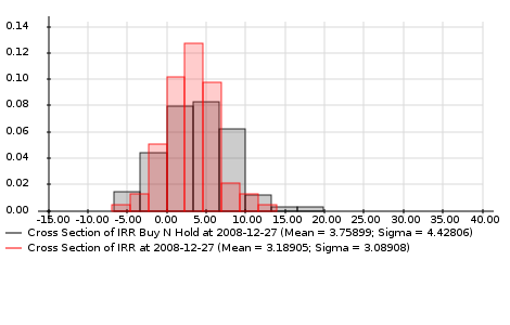
Monte Carlo test of the strategy
The real test of an investment strategy comes not from testing it against a specific period. To test the strategy I generated 100 "possible" S&P500 scenarios and checked how our strategy performs. The scenarios are generated using a GARCH stochastic volatility model. The model was calibrated using the parameters from Table 7 in the paper Maximum Likelihood Estimation of Stochastic Volatility Models by Y. Ait-Sahalia and R. Kimmel.
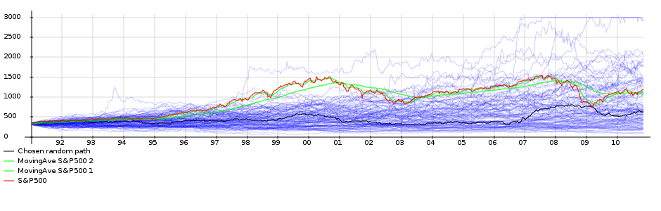
The final result is shown below. For each scenario we run our strategy and compare the internal rate of return of the strategy with the return we would have obtained with buy-and-hold. We find that the average return of our strategy over all scenarios is 3.19%, while the buy-and-hold strategy has an average return of 3.75%. However, the returns of our strategy are more consistent (lower standard deviation of returns): a buy-and-hold sometimes gives rise to very high returns, but also to more worse returns.
This conclusion is that I found for all the different (but similar) strategies that I have tested: a lower average return, but less risk (less extreme losses and gains).